
Students are asked to graph, or write an equation from, a polynomial function after identifying the characteristics of that polynomial function. This page is provided to assist a student accomplishing these tasks.
Contents
- Anatomy of a Polynomial Function
- Shape
- Graphs of Polynomial Functions
- Graphing a Polynomial Equation
- Writing an Equation from a Polynomial Graph
- Concavity
- References
- Additional Reading
Anatomy of a Polynomial Function
Polynomial functions (we usually just say “polynomials”) are used to model a wide variety of real phenomena. [1]

Shape
Exponent of the Leading Term ≥ 2n, where n ≥ 1

In the graph above, please note three facts as the value of the exponent increases.
- The y-value of decreases and the quadratic flattens for x = {x ∈ ℝ : 0 < x < 1} and x = {x ∈ ℝ : -1 < x < 0}.
- The “legs” of the quadratic get closer to vertical (i.e., the y-value increases) for x = {x ∈ ℝ : x < -1} and x = {x ∈ ℝ : x > 1}.
- The y value at x = 1 and x = -1 remains constant, i.e., (1, 1) and (-1, 1), respectively.
Exponent of the Leading Term ≥ 2n+1, where n ≥ 1
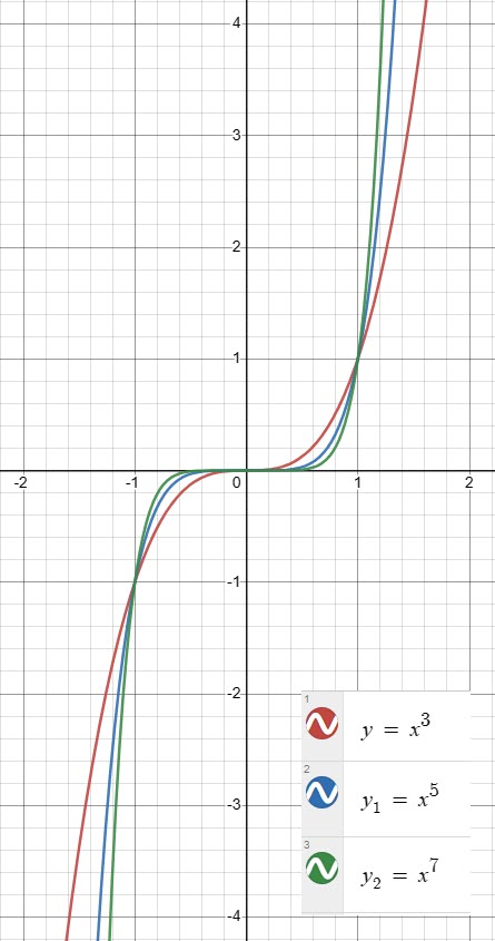
In the graph above, please note three facts as the value of the exponent increases.
- The y-value of decreases and the cubic flattens for x = {x ∈ ℝ : 0 < x < 1} and x = {x ∈ ℝ : -1 < x < 0}.
- The “legs” of the cubic get closer to vertical (i.e., the y-value increases) for x = {x ∈ ℝ : x < -1} and x = {x ∈ ℝ : x > 1}.
- The y value at x = 1 and x = -1 remains constant, i.e., (1, 1) and (-1, 1), respectively.
Graphs of Polynomial Functions
Each algebraic feature of a polynomial equation has a consequence for the graph of the function. Here is a table of those algebraic features, such as single and double roots, and how they are reflected in the graph of f(x). [1]
| Term | Definition |
|---|---|
| Single root | A solution of f(x) = 0 where the graph crosses the x-axis. For example, the quadratic function f(x) = (x+2)(x-4) has single roots at x = -2 and x = 4. |
| Double root | A solution of f(x) = 0 where the graph just touches the x-axis and turns around (creating a maximum or minimum – see below). For example, the cubic function f(x) = (x-2)2(x+5) has a double root at x = 2 and a single root at x = -5. |
| Triple root | A solution of f(x) = 0 where the graph crosses the x-axis and the curvature changes sign. See the graph below. For example, the cubic function f(x) = x3 has a triple root at x = 0. |
| Inflection point | The name of the point that is a triple root of a polynomial function. The curvature of the graph changes sign at an inflection point between concave-upward and concave-downward. Not all inflection points are located at triple roots (or even at roots at all), but all triple roots are inflection points located on the x-axis. |
| y-intercept | The solution to f(0); the point where a graph crosses the y-axis, usually a convenient (and very easy-to-find) point to plot when sketching a graph. |
| Local maximum & minimum | When a graph turns around (up to down or down to up), a maximum or minimum value is created. Local maxima or minima are not the highest or lowest points on a graph. |
| Global maximum & minimum | The parabola f(x) = x2 has a global minimum at x = 0, but no global maximum (it increases without bound). The parabola f(x) = -x2 has a global maximum, but no global minimum. The graph below has a global maximum at x = 1. The highest/lowest point on a graph (one may not exist). |
| End behavior | When x is large, either positive or negative, we are concerned with whether the function increases or decreases without bound (it will do one or the other). |
The appearance of the graph of a polynomial is largely determined by the leading term – it’s exponent and its coefficient. Because the leading term has the largest power, its size outgrows that of all other terms as the value of the independent variable grows. For example, in f(x)=8x4−4x3+3x2−2x+22, as x grows, the term 8x4 dominates all other terms.
You can check this out yourself by making a quick spreadsheet. Label one column x and fill it with integer values from 1-10, then calculate the value of each term (4 more columns) as x grows. Sum them and add the constant term (22) to find the value of the polynomial. The leading term will grow most rapidly. Here’s what I mean: [1]


It is important that you become adept at sketching the graphs of polynomial functions and finding their zeros (roots), and that you become familiar with the shapes and other characteristics of their graphs. [1]
Graphing a Polynomial Equation
Graphing Steps
Graphing a polynomial function involves the following steps.
- Factor the polynomial (if needed)
- Greatest common factor (GCF)
- Factoring by grouping
- Recognizing the form of a quadratic
- Recognizing the form of a quadratic
- The rational root theorem
- Determine the End Behavior by examining the leading term (see the Leading Coefficient Test).
- Find the intercepts and use the multiplicities of the zeros to determine the behavior of the polynomial at the x-intercepts.
- Use the end behavior and the behavior at the intercepts to sketch a graph.
- Optionally …
- Check for symmetry. If the function is an even function, its graph is symmetrical about the y-axis, that is, f(−x) = f(x) . If a function is an odd function, its graph is symmetrical about the origin, that is, f(−x) = −f(x).
- Ensure that the number of turning points does not exceed one less than the degree of the polynomial.
- Use technology (e.g., Desmos or a graphing calculator) to check the graph.
Graphing Example
See Polynomials II for an example using the above steps.
Writing an Equation from a Polynomial Graph
Now that we know how to find zeros of polynomial functions, we can use them to write formulas based on graphs. Because a polynomial function written in factored form will have an x-intercept where each factor is equal to zero, we can form a function that will pass through a set of x-intercepts by introducing a corresponding set of factors.
Equation Steps
First, notice that the graph is nice and smooth. There are no holes or breaks in the graph and there are no sharp corners in the graph. The graphs of polynomials will always be nice smooth curves. [2]
Secondly, the “humps” where the graph changes direction from increasing to decreasing or decreasing to increasing are often called turning points. If we know that the polynomial has degree n then we will know that there will be at most n−1 turning points in the graph. [2]
- Identify the x-intercepts of the graph to find the factors of the polynomial.
- Examine the behavior of the graph at the x-intercepts to determine the multiplicity of each factor. Use the multiplicity to determine if the x-intercept that corresponds to each zero will cross the x-axis or just touch it and if the x-intercept will flatten out or not.
- Find the polynomial of least degree containing all of the factors found in the previous step.
- Use any other point on the graph (the y-intercept may be easiest) to determine the stretch factor.
Equation Example
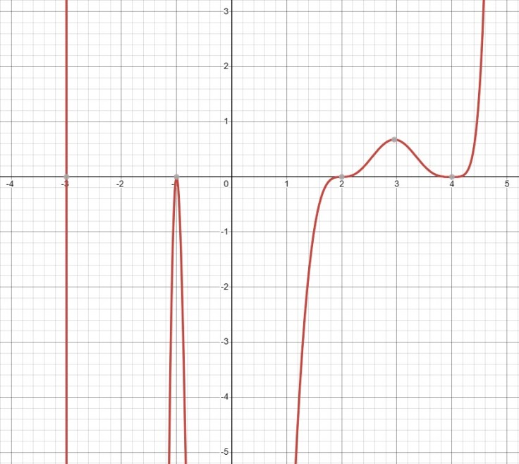
The graph above shows a tenth-degree polynomial with all real-number roots.
- The x-intercepts from the example graph are at -3, -1, 2 and 4.
- The respective multiplicities of each x-intercept is p=1 (crosses the x-axis), p=2 (touches or is tangent to the x-axis), p=3 (passes through the x-axis at the intercept but flattens out a bit first) and p=4 (touches or is tangent to the x-axis but is flatter). Since the sum of the multiplicities must be 10 (given in statement above), the multiplicity of x = 4 must have a multiplicity grater than 2, i.e., 4. [4]
- Find the polynomial of least degree containing all of the factors found in the previous step.
- Using the above information we have f(x) = (x-4)4(x-2)3(x+1)2(x+3)
- However, the function does not match the graph exactly. Therefore, we need to see if there is a scale factor.
- Use any the y-intercept for the function with and without the scale factor to determine the stretch factor.
- y-intercept with Scale Factor: (x, y) = (0, —61.44)
- y-intercept without Scale Factor: (x, y) = (0, —6144) (We can estimate the y-intercept by visually examining the graph in Desmos and see where the graph crosses the x-axis..)
- Stretch Factor: 0.01
Therefore, we have the final function f(x) = 0.01(x-4)4(x-2)3(x+1)2(x+3), or expanded as
f(x) = 0.01(x10 – 17x9 + 101x8 – 163x7 – 726x6 + 3372x5 – 3352x4 – 4864x3 + 9472x2 + 1024x – 6144)
Concavity
How does the second derivative test help determine the concavity of a function if the first derivative test already gives us the relative minimum/maximum? [5]
Just read through it and you will see when the curve is concave up or down.
References
[1] ⭐ “Polynomial Functions”. 2023. xaktly.com. https://xaktly.com/MathPolynomial.html.
xaktly.com by Dr. Jeff Cruzan is licensed under a Creative Commons Attribution-NonCommercial-ShareAlike 3.0 Unported License. © 2012, Jeff Cruzan. All text and images on this website not specifically attributed to another source were created by me and I reserve all rights as to their use. Any opinions expressed on this website are entirely mine, and do not necessarily reflect the views of any of my employers.
[2] “Algebra – Graphing Polynomials”. Section 5.3 : Graphing Polynomials. 2023. tutorial.math.lamar.edu. https://tutorial.math.lamar.edu/Classes/Alg/GraphingPolynomials.aspx.
[3] “Writing Formulas for Polynomial Functions”. 2023. Lumen Learning. https://courses.lumenlearning.com/waymakercollegealgebra/chapter/writing-formulas-for-polynomial-functions/.
[4] See the Degrees, Turnings, and “Bumps” web page for details on multiplicity, and check out the graphs on Desmos to see the difference in the graphs especially at x = 4. Also see the example graph, Exponent of the Leading Term ≥ 2n, where n ≥ 1, above.
[5] Lloyd, Philip. 2024. “How does the second derivative test help determine the concavity of a function if the first derivative test already gives us the relative minimum/maximum?” Quora. Accessed June 11. https://qr.ae/psDaXo.
Additional Reading
“Horizontal Compression – Properties, Graph, & Examples”. 2023. storyofmathematics.com. https://www.storyofmathematics.com/horizontal-compression/.
“Horizontal Stretch – Properties, Graph, & Examples”. 2023. storyofmathematics.com. https://www.storyofmathematics.com/horizontal-stretch/.
⭐ “How to Find Local Maxima and Minima: Explained with Examples.” 2023. GeeksForGeeks. https://www.geeksforgeeks.org/local-maxima-and-minima/amp/.
Local Maxima and Minima refer to the points of the functions, that define the highest and lowest range of that function. The derivative of the function can be used to calculate the Local Maxima and Local Minima. The Local Maxima and Minima can be found through the use of both the First derivative test and the Second derivative test.
In this article, we will discuss the introduction, definition, and important terminology of Local Maxima and Minima and its meaning. We will also understand the different methods to calculate the Local Maxima and Minima in mathematics and calculus. We will also solve various examples and provide practice questions for a better understanding of the concept of this article.
“Polynomials (Definition, Types and Examples)”. 2023. BYJUS. https://byjus.com/maths/polynomial/.
“Polynomials I”. 2022. Mathematical Mysteries. https://mathematicalmysteries.org/polynomials-i/.
- Adding and Subtracting Polynomials
- Multiplying Polynomials
- Dividing Polynomials
“Polynomials II”. 2022. Mathematical Mysteries. https://mathematicalmysteries.org/polynomials-ii/.
- Finding Zeros of a Polynomial Function
- Interpreting Turning Points
- Graphing a Polynomial Function
- Leading Coefficient Test
- End Behavior
- Multiplicity and Turning Points
“Polynomials III”. 2022. Mathematical Mysteries. https://mathematicalmysteries.org/polynomials-iii/.
- Factoring a Polynomial
- Greatest Common Factor
- Factoring by Grouping
- Factoring Polynomials in Quadratic Form
- Factoring Polynomials with Degree Greater than 2
“Polynomials IV”. 2022. Mathematical Mysteries. https://mathematicalmysteries.org/polynomials-iv/.
- Asymptotes
- Vertical Asymptotes
- Horizontal Asymptotes
- Holes of a Rational Function
“Polynomials V”. 2022. Mathematical Mysteries. https://mathematicalmysteries.org/polynomials-v/.
- Discontinuities
- Removeable (Hole)
- Non-Removeable
- Jump
- Infinite
- Endpoint
- Mixed
⭐ Stapel, Elizabeth. 2023. “Polynomial Graphs: End Behavior | Purplemath”. Purplemath. https://www.purplemath.com/modules/polyends.htm.
⭐ Stapel, Elizabeth. 2023. “Polynomial Graphs: Zeroes And Their Multiplicities | Purplemath”. Purplemath. https://www.purplemath.com/modules/polyends2.htm.
⭐ Stapel, Elizabeth. 2023. “Polynomial Graphing: Multiplicities Of Zeroes & “Flexing” | Purplemath”. Purplemath. https://www.purplemath.com/modules/polyends3.htm.
⭐ Stapel, Elizabeth. 2023. “Polynomial Graphing: Degrees, Turnings, And “Bumps” | Purplemath”. Purplemath. https://www.purplemath.com/modules/polyends4.htm.
⭐ Stapel, Elizabeth. 2023. “Quickie Graphing Of Polynomials | Purplemath”. Purplemath. https://www.purplemath.com/modules/polyends5.htm.
“Vertical Compression – Properties, Graph, & Examples”. 2023. storyofmathematics.com. https://www.storyofmathematics.com/vertical-compression/.
“Vertical Stretch – Properties, Graph, & Examples”. 2023. storyofmathematics.com. https://www.storyofmathematics.com/vertical-stretch/.
⭐ I suggest that you read the entire reference. Other references can be read in their entirety but I leave that up to you.
The featured image on this page is from the CUEMATH website.
